
14.1. Algorithms#
This section introduces algorithm foundations using a simple input-process-output model and more.
14.1.1. What Is an Algorithm?#
In short, an algorithm is a finite, ordered set of steps that transforms input into output. A useful mental model for algorithm therefore is:
Input: data provided to solve a problem
Process: the steps that operate on the data
Output: the result produced by the steps
A useful everyday analogy is a recipe: it specifies ingredients (inputs), a sequence of steps (instructions), and produces a dish (output). Like a recipe, an algorithm must eventually stop; it cannot run forever.
The flowchart below represents the concept of a computer algorithm.
         INPUT
           │
           ▼
    ┌──────────────┐
    │   STEP  1    │
    └──────┬───────┘
           │
           ▼
    ┌──────────────┐
    │   STEP  2    │
    └──────┬───────┘
           │
           ▼
    ┌──────────────┐        ┌─────────────┐
    │   STEP  3    │──YES──▶│  DO  THIS   │
    │  condition?  │        └─────────────┘
    └──────┬───────┘
           │ NO
           ▼
    ┌──────────────┐
    │   STEP  4    │◀─────────────┐
    └──────┬───────┘              │
           │                      │
           ▼                      │
    ┌──────────────┐              │
    │   loop?      │──────────────┘
    └──────┬───────┘
           │ done
           ▼
         OUTPUT
For example, you can design an algorithm to look through an array (in general sense) to find the largest value in an array; in this case, a Python list. Here, pretend that the max() function does not exist. For the example, suppose you want to go through the values in the array one by one. Check if the current value is the highest so far, and if it is, store it, then keep going until the end of the array. After looking at all the values, the stored value will be the highest of all values in the array.
A sketchy algorithm of the process just described may look like this:
Go through the elements and get the values in the array one by one.
Check if the current value is the highest so far, and if it is, store it.
After looking at all the values, the stored value will be the highest of all values in the array.
Why Algorithms in Python?
So by now you are probably thinking: Since Python has many built-in methods (max() in this case) that already serve as algorithms, why do you still need to learn algorithms in Python? Here’s why:
Built-in Algorithms:
Built-in methods like max(), sorted(), and sum() are convenient, but they are not a replacement for understanding algorithms. These methods are pre-implemented algorithms. Knowing how they work under the hood helps you understand their time and space complexity and recognize when they may be suboptimal or fail entirely. For example, max(my_list) still scans every element at \(O(n)\) and it does not magically run faster just because Python provides it.
Problem Coverage: Python built-ins do not cover all problem scenarios. Real-world challenges such as finding the shortest path in a network, scheduling tasks under constraints, recommending similar users, or detecting fraud patterns have no ready-made Python method. Solving them requires you to design and reason about algorithms from the ground up.
Algorithmic Thinking:
Even when built-ins exist, algorithmic thinking determines whether you can use them correctly and efficiently. Consider the difference between checking membership in a list versus a set: both work, but one runs in \(O(n)\) and the other in \(O(1)\). Without understanding the underlying algorithms, you cannot make that distinction, which matters enormously at scale. Similarly, calling max() inside a loop without realizing it re-scans the entire list each iteration can silently turn an \(O(n)\) problem into an \(O(n^2)\) one.
Problem-Solving: Finally, algorithms are the foundation of problem-solving and computational thinking. Built-in methods are tools, and algorithmic knowledge is what tells you which tool to use, why it works, what its limits are, and what to do when no tool exists. This is why most technical interviews include algorithm questions.
Overall, understanding algorithms therefore means understanding what those tools are actually doing, when they are fast or slow, and what to do when no built-in exists for your problem.
With the algorithm formulated, you may implement the algorithm in a specific programming language such as Python:
def max_value(nums):            ### input the array
    if not nums:                ### If the list is empty, return None
        return None             ### a "guard clause" to handle empty lists

    current_max = nums[0]       ### Initialize current_max to the first element of the list
    for x in nums[1:]:          ### Iterate through the list starting from the second element
        if x > current_max:     ### If the current element is greater than current_max, update current_max
            current_max = x
    return current_max          ### Return the maximum value found in the list

sample = [12, 4, 19, 7, 3]
print('input :', sample)
print('output:', max_value(sample))
input : [12, 4, 19, 7, 3]
output: 19
And this is probably how the Python max() function is defined. To make sure, the [Python Standard Library] has a description of the max() function and the implementation, written in C, is on github. An emulation of that implementation in Python looks like this (partial code). As you can see, the two versions are very comparable.
def mymax_backend(      ### T is a generic type; works with any comparable type (int, str, etc.)
    first_value: T,     ### The first value to compare against (the "current largest")
    it: Iterator[T],    ### The remaining elements as an iterator
    key: Optional[Callable[[T], Any]],
) -> T:
    largest = first_value
    if key is None:
        for x in it:
            if x > largest:
                largest = x
        return largest
    largest_key = key(largest)
    for x in it:
        kx = key(x)
        if kx > largest_key:
            largest = x
            largest_key = kx
    return largest
However, you have probably noticed that the algorithm is too sketchy to design both algorithms, and you need something more elaborate.
14.1.1.1. Properties of an Algorithm#
According to Donald Knuth in The Art of Computer Programming, an algorithm has certain properties:
Input: An algorithm starts in its initial state, which may be expressed as zero or more input values given before the algorithm starts.
Output: An algorithm will produce zero or more outputs in relation to the inputs.
Finiteness steps: An algorithm must start and stop with the rules the algorithm applies concluded. It cannot run forever; every algorithm must have a clear termination condition.
Definiteness: Each instruction in an algorithm must be precise and unambiguous; they cannot be open to interpretations. Every step must be clear enough that anyone or any machine can follow it without interpretation. For example, “iterate a bunch of times” is not well-defined; the number of times must be precisely expressed.
Effectiveness: The steps an algorithm takes must be sufficiently simple that they could be expressed; these steps must make sense for the quantities used.
You may also be concerned about some issues about algorithms such as:
Algorithms are not tied to any specific programming language. They describe what to do, not how a particular language does it.
Given the same input, an algorithm always produces the same output; this property is called determinism.
### Exercise: Find the Minimum Value
#   1. Write a function `find_min(nums)` that returns the minimum value
#      in a list WITHOUT using Python's built-in min() function.
#   2. Your algorithm should work for any non-empty list of numbers.
#   3. Test with: find_min([5, 2, 8, 1, 9, 3])  -> 1
### Your code starts here.


### Your code ends here.
1
10
-3
14.1.2. Implementing Algorithms#
An algorithm on paper is not yet a program. This section follows the path from a written algorithm to working, tested code, and shows the control patterns that most implementations are built from.
14.1.2.1. The Design Process#
Looking at the max_value() example, there is a gap between having an algorithm figured out and having a piece of code to run and test the algorithm for correctness and efficiency. To jump from a sketchy algorithm to code may not be as easy as you want it to be as the steps are not “well-defined”. Therefore, before implementing the algorithm using an actual programming language, it is usually smart to first write the algorithm as a step-by-step procedure.
So, before coding, you might want to use a design checklist like this:
Define input types and output format.
Write step-by-step logic in plain language.
Choose data structures that support the operations you need.
Test edge cases first (empty input, single item, duplicates, min/max, out of bound (0, -1, …), etc).
Measure performance only after correctness is confirmed.
For the design of the algorithm, if you can write down the algorithm in something between human language and programming language, the algorithm will be easier to implement later because you avoid drowning in all the details of the programming language syntax. The max_value() function algorithm can look like this:
Create a variable
maxValand set it equal to the first value of the array. (Variable)Go through every element in the array. (Iteration)
If the current element has a higher value than
maxVal, updatemaxValto this value. (Update)After looking at all the elements in the array, the
maxValvariable now contains the highest value.
In addition, you may choose to express this procedure in pseudo code, which should further define the steps of an algorithm.
Variable 'maxVal' = array[0]
For each element in the array
    If current element > maxVal
        maxVal = current element
14.1.2.2. Control Patterns#
In computer science, computer scientists evaluate algorithms on two key dimensions:
Correctness: does it produce the right answer for all valid inputs, including edge cases?
Efficiency: how much time and memory does it consume as the input grows? This is formalized through complexity analysis, commonly expressed using Big \(O\) notation such as \(O(n)\) or \(O(n^2)\).
Once the algorithm is correct, attention shifts to efficiency. To achieve efficiency, the design involves decisions about data structures and performance measurement. While going through these steps of the checklist, you want to pay attention to the three control patterns that most algorithms use to achieve better efficiency:
Sequence: These steps run in order, one after another, with no branching or looping. This is the simplest pattern: each line executes exactly once, in the order it appears. For example, initializing a variable and then returning it are two sequential steps.
Decision: choose different paths based on a condition (
if/elif/else). Decisions let an algorithm respond differently to different inputs. For example, returningNonefor an empty list (guard clause) or assigning a letter grade based on a score are both decisions.Repetition: repeat a block of work for each item in a collection, or until a condition is met (
for,while). Repetition lets an algorithm scale to any input size without duplicating code. For example, scanning every element in a list to find the maximum value uses repetition.
These three building blocks are enough to express the logic of virtually any algorithm. In practice, most algorithms layer all three: repetition drives the overall traversal, decisions handle special cases inside, and sequence connects each step in the right order.
Observe the following code and see the three building blocks of an algorithm.
def classify_scores(scores):
    labels = []
    for s in scores:                      # repetition
        if s >= 90:                       # decision
            labels.append('A')
        elif s >= 80:
            labels.append('B')
        else:
            labels.append('C')
    return labels                         # sequence (line #2, 3, 10) ends with output

print(classify_scores([95, 81, 72, 90]))
['A', 'B', 'C', 'A']
Another example for observing the three building blocks of an algorithm.
def summarize_orders(orders, discount_threshold=100):
    total_revenue = 0                           ### sequence: initialize output
    discounted_count = 0                        ### sequence: initialize counter

    for order in orders:                        ### repetition: visit every order
        amount = order['amount']

        if amount >= discount_threshold:        ### decision: qualify for discount?
            amount *= 0.9                       ### sequence: apply 10% discount
            discounted_count += 1               ### sequence: track how many

        total_revenue += amount                 ### sequence: accumulate

    return total_revenue, discounted_count      ### sequence: produce output
### Exercise: Count Passing Scores
#   1. Write a function `count_passing(scores)` that returns the count of
#      scores that are 60 or above.
#   2. Your function must use all three control patterns:
#      sequence, selection (if), and repetition (for).
#   3. Test with: count_passing([45, 72, 60, 88, 55])  -> 3
### Your code starts here.


### Your code ends here.
3
0
3
14.1.3. Complexity and Big O#
When evaluating an algorithm, correctness always comes first: the algorithm must produce the right answer for all valid inputs, including edge cases, before efficiency is even worth considering. A fast algorithm that gives wrong answers is not useful.
Once correctness is established, efficiency becomes the next concern. Big \(O\) notation is the standard way to describe how an algorithm’s runtime (or memory usage) grows as the input size \(n\) increases. It captures the shape of the growth: not the exact number of operations, but whether the algorithm scales linearly, logarithmically, quadratically, and so on. This allows you to compare algorithms independent of hardware or implementation details.
14.1.3.1. Complexity#
In algorithm analysis, Big \(O\) notation expresses the concept of complexity, which usually comes in two kinds:
time complexity (how runtime grows with input size) and
space complexity (how extra memory usage grows with input size).
This chapter focuses primarily on time complexity for search and sorting.
Earlier chapters briefly addressed Big \(O\) notation. You already compared item in list (often \(O(n)\)) with item in dict/set (average \(O(1)\)); see Big O Notation (dict) and Big O Notation (set). This section extends that foundation to \(O(\log n)\), \(O(n \log n)\), and \(O(n^2)\) for search and sorting algorithms.
The most common growth classes in algorithm analysis include:
Notation |
Class |
Behavior |
Example |
|---|---|---|---|
\(O(1)\) |
Constant |
Runtime does not depend on input size |
Dict/set lookup, list indexing |
\(O(\log n)\) |
Logarithmic |
Input is halved each step; doubles only when input squares |
Binary search |
\(O(n)\) |
Linear |
One pass through the data; grows proportionally with input |
Linear search, |
\(O(n \log n)\) |
Linearithmic |
Repeated splitting and merging; typical of efficient sorts |
Merge sort, Timsort |
\(O(n^2)\) |
Quadratic |
Nested loops over the input; impractical for large \(n\) |
Insertion/bubble sort |
The following examples illustrate each Big \(O\) class with a concrete, runnable implementation. The subsection Searching as a Complexity Example, later in this section, then compares \(O(n)\) and \(O(\log n)\) directly.
14.1.3.2. Big-O Complexity Overview#
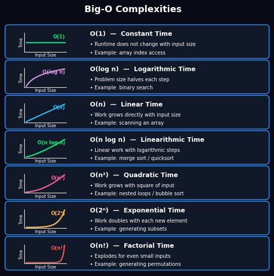
The chart below summarizes the seven most common Big-O growth rates, from fastest to slowest.
### O(1) — Constant: runtime does not depend on input size
scores = {'Alice': 95, 'Bob': 82}
grade = scores['Alice']                       # dict lookup: same cost for 10 or 10 million items
print(f"O(1) \t\t dict lookup → {grade}")


### O(n) — Linear: one pass through the data
def linear_max(arr):
    best = arr[0]
    for val in arr:                           # visits every element once
        if val > best:
            best = val
    return best

print(f"O(n) \t\t linear max → {linear_max([3, 7, 1, 9, 4])}")


### O(log n) — Logarithmic: binary search halves the search space each step
def binary_search(arr, target):
    lo, hi = 0, len(arr) - 1
    while lo <= hi:
        mid = (lo + hi) // 2
        if arr[mid] == target:
            return mid
        elif arr[mid] < target:
            lo = mid + 1
        else:
            hi = mid - 1
    return -1

sorted_nums = list(range(1_000_000))
print(f"O(log n) \t binary search → index {binary_search(sorted_nums, 999_999)}")


### O(n log n) — Linearithmic: Python's built-in sort (Timsort)
data = [5, 2, 9, 1, 7, 3]
print(f"O(n log n) \t sorted → {sorted(data)}")


### O(n²) — Quadratic: bubble sort with nested loops over the same input
def bubble_sort(arr):
    arr = arr[:]
    n = len(arr)
    for i in range(n):                        # outer loop: n passes
        for j in range(n - i - 1):           # inner loop: up to n comparisons each pass
            if arr[j] > arr[j + 1]:
                arr[j], arr[j + 1] = arr[j + 1], arr[j]
    return arr

print(f"O(n²) \t\t bubble sort → {bubble_sort([5, 2, 9, 1, 7, 3])}")
O(1) 		 dict lookup → 95
O(n) 		 linear max → 9
O(log n) 	 binary search → index 999999
O(n log n) 	 sorted → [1, 2, 3, 5, 7, 9]
O(n²) 		 bubble sort → [1, 2, 3, 5, 7, 9]
14.1.3.3. Searching as a Complexity Example#
Searching gives you a concrete way to compare two growth rates. Suppose you need to find a number in a sorted list of the values 1 to \(n\).
Linear search checks the items one at a time from the left. In the worst case (the target is last or absent), it inspects all \(n\) items, so its time complexity is \(O(n)\): doubling the list doubles the work.
Binary search checks the middle item of a sorted list and discards the half that cannot contain the target. Each comparison halves the remaining range, so the worst case needs \(\lfloor \log_2 n \rfloor + 1\) comparisons, which is \(O(\log n)\): doubling the list adds only one step.
The cell below computes the worst-case step counts from these two formulas without running either search.
import math

print(f"{'n':>13}  {'linear':>13}  {'binary':>6}")
for n in [10, 100, 1_000, 1_000_000, 1_000_000_000]:
    linear_steps = n                              # O(n): check every item
    binary_steps = math.floor(math.log2(n)) + 1   # O(log n): halve until one item is left
    print(f"{n:>13,}  {linear_steps:>13,}  {binary_steps:>6}")
            n         linear  binary
           10             10       4
          100            100       7
        1,000          1,000      10
    1,000,000      1,000,000      20
1,000,000,000  1,000,000,000      30
The gap widens as \(n\) grows. For one billion items, a linear scan may need a billion comparisons, while binary search needs at most 30. Binary search pays for this speed with a requirement: the input must be sorted, and sorting costs \(O(n \log n)\).
For the implementations, hand traces, the bisect module, hash-based lookup, and timing experiments, see 14.2 Searching.
### Exercise: Identify the Big O Class
#   For each function below, write (as a comment) its time complexity
#   in Big O notation and a one-line reason.
#   1. def count_evens(nums):
#          return [n for n in nums if n % 2 == 0]
#   2. def first_item(nums):
#          return nums[0]
#   3. def has_duplicate(nums):
#          for i in range(len(nums)):
#              for j in range(i + 1, len(nums)):
#                  if nums[i] == nums[j]:
#                      return True
#          return False
### Your code starts here.


### Your code ends here.
n =    10:      45 comparisons
n =   100:   4,950 comparisons
n = 1,000: 499,500 comparisons
14.1.4. Benchmarking#
Benchmarking measures how long your code actually takes to run. It complements Big O analysis: Big O tells you the shape of growth asymptotically, while benchmarking gives you concrete runtimes on real hardware with real data. Together they answer both “will this scale?” and “is this fast enough today?”
Python provides three main tools for timing code, each suited to a different level of precision:
time.time(): Returns wall-clock time as a float (seconds since the Unix epoch). Acceptable for rough, one-off prints where precision doesn’t matter, but it can be skewed by OS clock corrections.time.perf_counter(): Returns a high-resolution performance counter with sub-microsecond precision. It is unaffected by OS clock changes, making it the preferred choice for timing short code blocks in instrumented scripts.timeit.timeit()/timeit.repeat(): The right tool for microbenchmarking a single expression or small snippet. It disables garbage collection between runs to reduce noise, executes the code many times to average out fluctuations, and manages multiple trials automatically. Use this when you need a repeatable, statistically meaningful measurement of a specific line or expression.
Function |
Module |
Resolution |
Use For |
Notes |
|---|---|---|---|---|
|
|
Low (~10ms) |
Timestamps, logging, wall-clock elapsed |
Can go backward if system clock adjusted |
|
|
Very high (ns) |
Benchmarking code blocks |
Best for measuring elapsed time; never goes backward |
|
|
Very high (ns) |
Microbenchmarks: single expression or function |
Runs |
|
|
Very high (ns) |
Microbenchmarks across multiple trials |
Returns list of times; use |
The code below times the same operation, max(data) on a list of 100,000 numbers, with each of the four tools, so you can compare how each one is called and what it reports.
import time
import timeit

data = list(range(100_000))

### --- time.time() --- for timestamps, logging,
# Coarse wall-clock timing; fine for quick prints, not precision work.
start = time.time()
max(data)
end = time.time()
print(f"time.time()        : {end - start:.6f} s")

### --- time.perf_counter() --- for benchmarking code performance.
# High-resolution counter; preferred for timing instrumented code blocks.
start = time.perf_counter()
max(data)
elapsed = time.perf_counter() - start
print(f"perf_counter()     : {elapsed:.6f} s")

### --- timeit.timeit() ---
# Runs the snippet many times and returns total time; best for microbenchmarks.
t = timeit.timeit(lambda: max(data), number=1_000)
print(f"timeit (1000 runs) : {t:.4f} s total  |  {t/1000*1e6:.2f} µs per call")

### --- timeit.repeat() ---
# Like timeit() but returns a list of times across multiple trials; use min() to report.
trials = timeit.repeat(lambda: max(data), repeat=5, number=200)
print(f"timeit.repeat()    : best of 5 trials = {min(trials)/200*1e6:.2f} µs per call")
time.time()        : 0.001096 s
perf_counter()     : 0.001127 s
timeit (1000 runs) : 1.1883 s total | 1188.26 µs per call
timeit.repeat() : best of 5 trials = 1190.08 µs per call
Why Use lambda with timeit?
Here, lambda functions defer the execution of max(data) until timeit calls it.
If you had written
timeit.timeit(max(data), number=1000)
then max(data) runs once immediately and returns a number (e.g. 99999). Then timeit tries to call 99999 1000 times, which crashes. The lambda wraps it into a zero-argument function that timeit can call over and over:
t = timeit.timeit(lambda: max(data), number=1_000)
#                 ^^^^^^
#                 callable — timeit calls this 1000 times
#                 each call runs max(data) fresh
This is the same as:
def run():
    return max(data)

t = timeit.timeit(run, number=1_000)   # same thing, no lambda
The lambda is just a compact way to write that one-liner inline. The pattern lambda: <expression> is the standard idiom for “wrap this expression so it can be called later.”
### Exercise: Benchmark List vs. Set Membership
#   1. Create a list `data` with integers 0 to 99,999.
#   2. Create a set `data_set` from the same values.
#   3. Use timeit to measure 1000 lookups of 99999 in each.
#   4. Print both times and state which is faster.
### Your code starts here.


### Your code ends here.
List lookup: 0.6970s
Set  lookup: 0.0000s
Set is ~14616x faster
14.1.5. Algorithm Selection Guide#
Use this table as a quick reference when choosing a strategy:
Condition |
Recommended Approach |
Complexity |
|---|---|---|
Unsorted data, few lookups |
Linear search |
\(O(n)\) |
Sorted data, repeated lookups |
Binary search |
\(O(\log n)\) |
Heavy membership checks on static data |
|
\(O(1)\) average |
Nearly sorted input |
Insertion sort |
\(O(n)\) best case |
General-purpose sort |
Merge sort / Python Timsort |
\(O(n \log n)\) |
### Exercise: Choose the Right Algorithm
#   For each scenario, write (as a comment) the recommended approach
#   and its Big O complexity.
#   1. A sorted list of 1 million product IDs -- find a specific ID.
#   2. An unsorted list of 10 names -- find one name.
#   3. Repeated membership checks on a static collection of usernames.
#   4. A nearly sorted list of timestamps -- sort them.
### Your code starts here.


### Your code ends here.
alice: member
eve: not a member
bob: member