Recursion

4.3. Recursion#

Recursion is a fundamentally different way of thinking about problems — decomposing into “solve a smaller version of the same problem” rather than iterating with loops. Many real problems (tree/graph traversal, divide-and-conquer algorithms, parsing nested structures) are naturally recursive and awkward to express iteratively.

Also, recursion is a prerequisite concept for later CS topics — recursive data structures (trees, linked lists), algorithms (quicksort, mergesort, binary search), and dynamic programming.

The general syntax for recursion in Python is:

def function_name(parameters):
    if base_case_condition:
        return base_case_value
    else:
        return function_name(smaller_parameters)

In this syntax, we see:

Base case: A condition that stops the recursion (no further recursive call). Without one, you get infinite recursion and eventually a RecursionError.
Recursive case: The function calls itself with an argument that moves toward the base case (usually smaller/simpler).
Progress: Each call must actually get closer to the base case, or it never terminates.

It is legal for a function to call itself. It may not be obvious why that is a good thing, but it turns out to be one of the most magical things a program can do. Here’s an example.

def countdown(n):
    if n <= 0:
        print('Blastoff!')
    else:
        print(n)
        countdown(n-1)

If n is 0 or negative, countdown outputs the word, “Blastoff!” Otherwise, it outputs n and then calls itself, passing n-1 as an argument.

Here’s what happens when we call this function with the argument 3.

countdown(3)

3
2
1
Blastoff!

The execution of countdown begins with n=3, and since n is greater than 0, it displays 3, and then calls itself…

The execution of countdown begins with n=2, and since n is greater than 0, it displays 2, and then calls itself…

The execution of countdown begins with n=1, and since n is greater than 0, it displays 1, and then calls itself…

The execution of countdown begins with n=0, and since n is not greater than 0, it displays “Blastoff!” and returns.

The countdown that got n=1 returns.

The countdown that got n=2 returns.

The countdown that got n=3 returns.

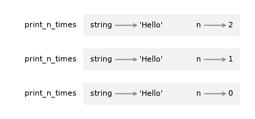
A function that calls itself is recursive. As another example, we can write a function that prints a string n times.

def print_n_times(string, n):
    if n > 0:
        print(string)
        print_n_times(string, n-1)

If n is positive, print_n_times displays the value of string and then calls itself, passing along string and n-1 as arguments.

If n is 0 or negative, the condition is false and print_n_times does nothing.

Here’s how it works.

print_n_times('Spam ', 4)

Spam 
Spam 
Spam 
Spam 

For simple examples like this, it is probably easier to use a for loop. But we will see examples later that are hard to write with a for loop and easy to write with recursion, so it is good to start early.

4.3.1. Stack diagrams for recursive functions #

Here’s a stack diagram that shows the frames created when we called countdown with n = 3.

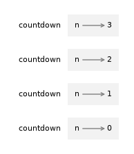
../../_images/f77f5b16cb68a34db5ffee1a7ed2742475fe19cb14afb6870f721be708365be6.png

The four countdown frames have different values for the parameter n. The bottom of the stack, where n=0, is called the base case. It does not make a recursive call, so there are no more frames.

../../_images/c6273db3d9605f60cd12d36076df15f716ba20ecad4f650d635a3ec11142c77c.png

### Exercise: Trace the Base Case
# Before running the code, predict the order of printed lines.
# Then run it and compare the output with your prediction.
def trace_countdown(n):
    print(f"enter {n}")
    if n <= 0:
        print("base case")
    else:
        trace_countdown(n - 1)
    print(f"leave {n}")

trace_countdown(3)

enter 3
enter 2
enter 1
enter 0
base case
leave 0
leave 1
leave 2
leave 3

enter 3
enter 2
enter 1
enter 0
base case
leave 0
leave 1
leave 2
leave 3

4.3.2. Infinite recursion #

If a recursion never reaches a base case, it goes on making recursive calls forever, and the program never terminates. This is known as infinite recursion, and it is generally not a good idea. Here’s a minimal function with an infinite recursion.

def recurse():
    recurse()
    
# recurse()  # Uncommenting this line will cause a RecursionError due to infinite recursion.

Every time recurse is called, it calls itself, which creates another frame. In Python, there is a limit to the number of frames that can be on the stack at the same time. If a program exceeds the limit, it causes a runtime error.

%xmode Context

Exception reporting mode: Context

try:
    recurse()
except RecursionError as error:
    print(type(error).__name__)

RecursionError

The traceback indicates that there were almost 3000 frames on the stack when the error occurred.

If you encounter an infinite recursion by accident, review your function to confirm that there is a base case that does not make a recursive call. And if there is a base case, check whether you are guaranteed to reach it.

### Exercise: Add a Stopping Condition
# The function below would recurse forever if it called itself unconditionally.
# Add a base case so it returns the number of steps needed to reach zero.
def steps_to_zero(n):
    pass

# Test your function with: print(steps_to_zero(4))

4.3.3. Recursion with return values #

Now that we can write functions with return values, we can write recursive functions with return values, and with that capability, we have passed an important threshold – the subset of Python we have is now Turing complete, which means that we can perform any computation that can be described by an algorithm because it has:

Conditional branching (if/else)
Some form of repetition (loops or recursion)
A way to read/write to unbounded memory (variables, data structures)

To demonstrate recursion with return values, we’ll evaluate a few recursively defined mathematical functions. A recursive definition is similar to a circular definition, in the sense that the definition refers to the thing being defined. A truly circular definition is not very useful:

vorpal: An adjective used to describe something that is vorpal.

If you saw that definition in the dictionary, you might be annoyed. On the other hand, if you looked up the definition of the factorial function, denoted with the symbol \(!\), you might get something like this:

\[\begin{split}\begin{aligned} 0! &= 1 \\ n! &= n~(n-1)! \end{aligned}\end{split}\]

This definition says that the factorial of \(0\) is \(1\), and the factorial of any other value, \(n\), is \(n\) multiplied by the factorial of \(n-1\).

../../_images/fibonacci.png — Fig. 4.1 Fibonacci Sequence#

If you can write a recursive definition of something, you can write a Python program to evaluate it. Following an incremental development process, we’ll start with a function that take n as a parameter and always returns 0.

def factorial(n):
    return 0

Now let’s add the first part of the definition – if the argument happens to be 0, all we have to do is return 1:

def factorial(n):
    if n == 0:
        return 1
    else:
        return 0

Now let’s fill in the second part – if n is not 0, we have to make a recursive call to find the factorial of n-1 and then multiply the result by n:

def factorial(n):
    if n == 0:
        return 1
    else:
        recurse = factorial(n-1)
        return n * recurse

factorial(5)

The flow of execution for this program is similar to the flow of countdown earlier in this section. If we call factorial with the value 3:

Since 3 is not 0, we take the second branch and calculate the factorial of n-1…

Since 2 is not 0, we take the second branch and calculate the factorial of n-1…

Since 1 is not 0, we take the second branch and calculate the factorial of n-1…

Since 0 equals 0, we take the first branch and return 1 without making any more recursive calls.

The return value, 1, is multiplied by n, which is 1, and the result is returned.

The return value, 1, is multiplied by n, which is 2, and the result is returned.

The return value 2 is multiplied by n, which is 3, and the result, 6, becomes the return value of the function call that started the whole process.

The following figure shows the stack diagram for this sequence of function calls.

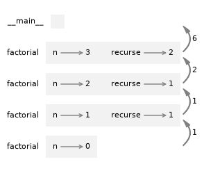
../../_images/9f985f3482febe5592a40ed5501a7c9fe824a216f87778ecf5f814eb8cb129c3.png

The return values are shown being passed back up the stack. In each frame, the return value is the product of n and recurse.

In the last frame, the local variable recurse does not exist because the branch that creates it does not run.

4.3.3.1. Recursion on Lists #

The same structure works on a list. A list can be split into two parts: its first item, items[0], and the rest of the list, items[1:]. The slice items[1:] is a new list that holds every item except the first, so it is one item shorter. That split gives a natural recursive definition:

Base case: an empty list. not items is True when items is empty, so the function can return without recursing.
Recursive case: handle the first item, then call the function on the rest of the list. Because the rest is always shorter, each call moves one step closer to the empty list.

As an example, here is a function that counts the items in a list without using len().

def count_items(items):
    if not items:                         ### base case: empty list
        return 0
    return 1 + count_items(items[1:])     ### 1 for the first item + count of the rest

fruits = ['apple', 'banana', 'cherry']
print(count_items(fruits))

Here is how the calls unfold for count_items(['apple', 'banana', 'cherry']):

count_items(['apple', 'banana', 'cherry'])
= 1 + count_items(['banana', 'cherry'])
= 1 + (1 + count_items(['cherry']))
= 1 + (1 + (1 + count_items([])))
= 1 + (1 + (1 + 0))                  <- base case returns 0
= 3

Each call removes one item until the list is empty. The base case returns 0, and the results are added up as each call returns, just as factorial multiplied its results on the way back up the stack. To process the items rather than only count them, replace the 1 with an expression that uses the first item, items[0].

### Exercise: Recursive Sum
# Write recursive_sum(nums), which returns the sum of a list of numbers.
# Hint: the sum of an empty list is 0; otherwise add the first item
# to the recursive sum of the rest of the list.
def recursive_sum(nums):
    pass

# Test your function with: print(recursive_sum([2, 4, 6, 8]))

4.3.4. Fibonacci #

After factorial, the most common example of a recursive function is fibonacci, which has the following definition:

\[\begin{split}\begin{aligned} \mathrm{fibonacci}(0) &= 0 \\ \mathrm{fibonacci}(1) &= 1 \\ \mathrm{fibonacci}(n) &= \mathrm{fibonacci}(n-1) + \mathrm{fibonacci}(n-2) \end{aligned}\end{split}\]

Translated into Python, it looks like this:

def fibonacci(n):
    if n == 0:
        return 0
    elif  n == 1:
        return 1
    else:
        return fibonacci(n-1) + fibonacci(n-2)

If you try to follow the flow of execution here, even for small values of \(n\), your head explodes. Rather than tracing every call, you can take a leap of faith: when you reach a recursive call, trust that it returns the correct result for the smaller input. If you assume that the two recursive calls work correctly, you can be confident that the last return statement is correct.

This way of computing Fibonacci numbers is very inefficient. The next section shows why, and how to fix it.

4.3.5. Memoization #

The recursive fibonacci is slow because it solves the same subproblems over and over. To compute fibonacci(5), it calls fibonacci(4) and fibonacci(3). But fibonacci(4) also calls fibonacci(3), so fibonacci(3) is computed twice, fibonacci(2) three times, and so on. The number of calls grows exponentially with n.

The cell below counts the calls needed to compute fibonacci(20):

calls = 0

def fibonacci_counted(n):
    global calls
    calls += 1
    if n < 2:
        return n
    return fibonacci_counted(n - 1) + fibonacci_counted(n - 2)

print(fibonacci_counted(20))
print(calls)

6765
21891

That is 21,891 calls to compute a single number. A better approach is to remember each result the first time it is computed and look it up after that. Storing previous results so they can be reused is called memoization (from “memo,” a note to yourself).

The version below keeps its results in a dictionary named known (dictionaries were previewed in 2.3 and are covered in Chapter 7). The dictionary starts with the two base cases. Before doing any work, the function checks whether the answer is already known:

known = {0: 0, 1: 1}
calls = 0

def fibonacci_known(n):
    global calls
    calls += 1
    if n in known:
        return known[n]
    result = fibonacci_known(n - 1) + fibonacci_known(n - 2)
    known[n] = result
    return result

print(fibonacci_known(20))
print(calls)

6765
39

Each Fibonacci number is now computed only once, so fibonacci(20) takes 39 calls instead of 21,891. The trade-off is memory: the dictionary keeps every result it has computed. Chapter 10 shows functools.lru_cache, which adds this kind of caching to a function automatically.

### Exercise: Memoized Fibonacci
# The plain recursive Fibonacci repeats a lot of work. Write fibonacci_memo(n)
# using the same pattern as fibonacci_known above: a global dictionary named
# memo that starts with the base cases. If n is already in memo, return memo[n];
# otherwise compute the result recursively, store it in memo, and return it.
memo = {0: 0, 1: 1}

def fibonacci_memo(n):
    pass

# Test your function with: print(fibonacci_memo(10)) and print(fibonacci_memo(50))

55
12586269025

4.3.6. When Not to Use Recursion #

Recursion is useful when a problem naturally breaks into smaller versions of itself, such as tree traversal or divide-and-conquer algorithms. In Python, recursion is not always the best default. Deep recursion can hit the recursion limit, and a simple loop is often clearer for linear repetition.

def factorial_loop(n):
    result = 1
    for value in range(2, n + 1):
        result *= value
    return result

print(factorial_loop(5))

Recursion

Contents

4.3. Recursion#

4.3.1. Stack diagrams for recursive functions#

4.3.2. Infinite recursion#

4.3.3. Recursion with return values#

4.3.3.1. Recursion on Lists#

4.3.4. Fibonacci#

4.3.5. Memoization#

4.3.6. When Not to Use Recursion#